3 Gravitational Wave Detection
Gravitational waves were first theorized by Einstein, accompanying his theory of general relativity. However, at the time it was not even clear whether they were an artifact of the theory or an observable phenomenon. Of course, as we have seen, Gravitational Wave (GW) are predicted to be extremely weak, and thus there was initially little hope of ever detecting them. As evidence mounted that General Relativity (GR) was indeed an incredibly accurate theory of gravity, the interest in GW detection grew. The first detectors, resonant antennas, failed in successfully detecting GW as they were simply not sensitive enough. The more modern laser based detectors were the finally able to claim detection, by being extremely sensitive (the modern measurement precision at Laser Interferometer Gravitational-Wave Observatory (LIGO) is equivalent to measuring the distance to Alpha Centauri 4.367 light-years, to the width of a human hair \(\sim 40~\mathrm{µm}\)). The first detection was made in 2015 [1], marking the beginning of a new era in astronomy, and maybe even physics itself.
3.1 Laser interferometers
Laser-interferometer-based GW detectors are essentially scaled-up versions of the Michelson interferometer. The device, shown in Figure 3.1, splits a beam of colimated coherent photons (laser) into two, letting them propagate along two axes in an L configuration, before being reflected back to the beam splitter. The two beams, when recombined, interfere with each other, constructively or destructively, depending on the nature of the medium they have traveled through and the length of each arm.
![]()
For a gravitational wave to produce a measurable effect on such an apparatus, all the optical equipment should be free to move and be isolated from external vibrations. This is achieved by hanging the mirror on precisely-tuned penduli. When the gravitational wave propagates through the apparatus, it induces a relative movement between the masses, changing the difference \(L_x-L_y\) in length of the detectors arms, by an amount \(\Delta L\). This effect is exacerbated as the length of the arms \(L_x \sim L_y \sim L\) is increased. It follows that the strain is the normalized difference:
\[ \frac{\Delta L}{L}=\left[(1 / 2)\left(1+\cos ^2 (\theta)\right) \cos (2 \phi)\right] h_{+}+[\cos (\theta) \sin (2 \phi)] h_{\times} \equiv h, \]
where \(\theta\) and \(\phi\) are the polar and azimuthal angles of the direction of propagation of the GW . The strain is decomposed into components, \(h_{+}\) and \(h_{\times}\), which are the plus and cross polarisations of the wave. The strain sensitivity can be further increased by bouncing the light back and forth multiple times along the arms of the interferometer. In current implementations this is achieved using Fabry - Perot cavities spanning the whole length of the arms.
3.1.1 LIGO and ground based observatories
LIGO implements the measurement apparatus described in the past section, and a schematic is shown in Figure 3.2. It consists of two detectors, both in the USA, one in Livingston Louisiana and one in Hanford Washington, a separation of \(3000 \text{ km}\). Each LIGO detector has two \(4\text{ km}\) long arms made up of \(1.2\text{ m}\)-wide vacuum tubes, each operating as Fabry-Perot cavities. The light from an effective \(750\text{ kW}\) laser bounces back and forth inside these arms around 300 times. Thus, the effective arm length becomes \(1200\text{ km}\), drastically improving sensitivity.
![]()
While LIGO was the first to provide detection data, it does not live in a vacuum. In fact for the first published detection, the data analysis teams from LIGO joined forces with those for Virgo, the European gravitational wave detector. The Virgo detector is located in Cascina, Italy, and is similar to LIGO . It has \(3\text{ km}\) long arms and a different suspension system. It joined data collection with LIGO in the second observing run in 2017. Finally, there are two other detectors that are now part of the collaboration, KAGRA in Japan and GEO600 in Germany. KAGRA is a similar detector to Virgo in scale, but is built underground further isolating it from seismic activity .GEO600 is a smaller detector, with \(600 \text{ m}\) long arms, built with the objective of being a test bed for future detectors.
Although they exhibit impressive sensitivity, ground based detectors are limited, since they are subject to seismic activity, which can cause vibrations that limits the lower bound of the frequency sensitivity of the detectors. The optics and other higher frequency noise imposes an upper bound to the frequency. In particular ground based detectors are only sensitive to frequencies in the following rough range:
\[ [10^{0},10^{4} ]\text{ Hz}. \]
In turn this implies that they are sensitive to the comparable, stellar mass 1 compact binaries, which are currently believed to be the most common type of binary systems in the universe. Of course this is not an accident, as these detectors were purpose built for providing evidence of GW in general. In fact, they have been quite successful in this regard, with upwards of 90 detections of GW to date.
1 and a bit bigger \(\sim 1 - 10^3 M_\odot\)
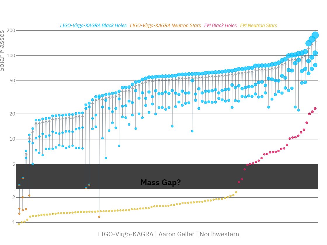
Figure 3.3 shows the current library of compact binary systems detected by LIGO -Virg-Kagra, along with those detected through GW means. The highlighted band denotes the assumed mass gap that should exist between the neutron star and black hole mass distributions. Note that most of the detections are compatible with the presence of such a gap. However, there are a few detections that are not, and these are particularly interesting. These are binaries with masses too light to be black holes, but too heavy to be neutron stars. A lot of research is ongoing to try and understand what these objects are, and if they are not just measurement artefacts.
3.1.2 Laser Interferometer Space Antenna (LISA)
There are many planned next generation GW detectors, from the Einstein telescope to Cosmic explorer. The most interesting one however is LISA the first genuine space based GW observatory. It is a joint project between ESA and NASA, and is scheduled to launch in 2037. In Figure 3.4 we see it will consist of three satellites, in triangular formation, at a distance of 2.5 million kilometers of each other. Each of the three LISA spacecraft contains a test mass free-falling within its body. Each spacecraft then measures the distance to its neighboring test mass thus forming a space based laser interferometer.
![]()
There are a few key differences with ground based detectors. The first is the size of the arms means it will be sensitive to frequency ranges such as:
\[ [10^{-4},10^{0} ]\text{ Hz}. \]
This means that it will be sensitive to the most massive binaries in the universe, supermassive black holes, such as those found at the centers of galaxies.
The second is that it will be completely isolated from seismic activity, and thus has a much lower noise floor. This combined with the arm length means that LISA is also predicted to be able to observe Extreme Mass Ratio Inspiral (EMRI) where stellar compact objects (\(<60 M_\odot\)) orbit around a massive black hole of around \(10^5 M_\odot\) or more. In this configuration the small mass is in a slowly decaying orbit, and thus can spend around \(10^5\) orbits and between a few months and a few years in the LISA sensitivity band before merging. This will provide us with a very interesting new source of GW , that also allows us to test new approximations, such as those based on mass ratio expansions: Gravitational Self-Force (GSF) .
3.2 Matched filtering
The signals measured by the laser interferometers such as LIGO , provide a measurement of strain over time. This waveform essentially measures the deformation of spacetime when a GW passes through a detector. While some GW signals observed in laser interferometers are clearly identified as such, mainly due to their extraordinary power output, weaker signals are harder to identify. In fact, most of the detections have happened under the noise floor of the detectors. How is this possible? Matched filtering and waveform generation.
Consider some detector output signal \(s\) consisting of noise \(n\) and a possible true GW signal \(h_i\) (or signals, making up a family \(\{h_i \}\)). The nature of the noise is unpredictable and necessarily probabilistic in nature. We can, however, model the noise as a random variable \(n\) that follows a probability distribution \(P_n\) dependent on variables that we consider and have measured to be significantly impactful.
In such a probabilistic setup one could try to find the probability that the signal \(h_i\in \{h_i \}\) has been detected, conditional on the actual data \(s\). This however is impractical as it requires a priori knowledge on the family of possible signals, information that is inaccessible. Instead, we devise a functional \(\mathcal{F}[s,h_i ]\), (a statistic) dependent on both the data and the supposedly present GW signal. We can then choose a threshold \(\rho^*\) above which we claim detection of the signal \(h_i\), i.e. if \(\mathcal{F}[s,h_i ]>\rho^*\).
The functional that is used is defined in terms of the symmetric inner product \(\langle s,h_i \rangle\), that correlates the data \(s\) with the template \(h_i\), weighting by detector frequency sensitivity \(S_n(f)\):
\[\langle g,h \rangle=2\int\limits_{-\infty}^{\infty}\frac{{\mathtip{\hat{g}}{\text{Fourier transform of $g$ in variable $x$: }{\hat{g}\left(2\pi f\right) = \int \,\mathrm{d}^{}x\, g(x) \texttip{\mathrm{e}^{\mathtip{\mathring{\imath}}{\text{Complex unit: } \mathring{\imath}^2 = -1}2\pi f \cdot x}}{exponential function}}}{}^\ast}(f)\mathtip{\hat{h}}{\text{Fourier transform of $h$ in variable $x$: }{\hat{h}\left(2\pi f\right) = \int \,\mathrm{d}^{}x\, h(x) \texttip{\mathrm{e}^{\mathtip{\mathring{\imath}}{\text{Complex unit: } \mathring{\imath}^2 = -1}2\pi f \cdot x}}{exponential function}}}(f)}{S_n(\vert f \vert)}\,\mathrm{d}^{}f\,=4 \Re{\int\limits_{0}^{\infty}}\frac{{\mathtip{\hat{g}}{\text{Fourier transform of $g$ in variable $x$: }{\hat{g}\left(2\pi f\right) = \int \,\mathrm{d}^{}x\, g(x) \texttip{\mathrm{e}^{\mathtip{\mathring{\imath}}{\text{Complex unit: } \mathring{\imath}^2 = -1}2\pi f \cdot x}}{exponential function}}}{}^\ast}(f)\mathtip{\hat{h}}{\text{Fourier transform of $h$ in variable $x$: }{\hat{h}\left(2\pi\right) = \int \,\mathrm{d}^{}x\, h(x) \texttip{\mathrm{e}^{\mathtip{\mathring{\imath}}{\text{Complex unit: } \mathring{\imath}^2 = -1}2\pi \cdot x}}{exponential function}}}(f)}{S_n({f})}\,\mathrm{d}^{}f\,,\]
where \({\mathtip{\hat{g}}{\text{Fourier transform of $g$ in variable $x$: }{\hat{g}\left(2\pi\right) = \int \,\mathrm{d}^{}x\, g(x) \texttip{\mathrm{e}^{\mathtip{\mathring{\imath}}{\text{Complex unit: } \mathring{\imath}^2 = -1}2\pi \cdot x}}{exponential function}}}{}^\ast}\) is the conjugate of the frequency Fourier transform of \(g\). \(S_n(f)\) is the noise power spectral density, characterising the detector sensitivity defined by:
\[ \overline{{\mathtip{\hat{n}}{\text{Fourier transform of $n$ in variable $x$: }{\hat{n}\left(2\pi f\right) = \int \,\mathrm{d}^{}x\, n(x) \texttip{\mathrm{e}^{\mathtip{\mathring{\imath}}{\text{Complex unit: } \mathring{\imath}^2 = -1}2\pi f \cdot x}}{exponential function}}}{}^\ast}(f_1)\mathtip{\hat{n}}{\text{Fourier transform of $n$ in variable $x$: }{\hat{n}\left(2\pi f\right) = \int \,\mathrm{d}^{}x\, n(x) \texttip{\mathrm{e}^{\mathtip{\mathring{\imath}}{\text{Complex unit: } \mathring{\imath}^2 = -1}2\pi f \cdot x}}{exponential function}}}(f_2)}=\tfrac{1}{2}\texttip{\delta^{{}}(f_1-f_2)}{Dirac delta function} S_n(f_1)\texttip{\Theta^{{}}(f_1)}{Heaviside step function}, \]
where the bar denotes the average over the noise realisation, \(\texttip{\delta^{{}}(f_1-f_2)}{Dirac delta function}\) is the Dirac delta function, and \(\texttip{\Theta^{{}}(f_1)}{Heaviside step function}\) is the Heaviside step function. We can now define the signal to noise ratio for the signal when filtered by \(h_i\) as 2
2 The equality is due to the fact that we average over all realisations of noise, which averages to uniform: \(\overline{\langle h_i,n \rangle\langle n,h_i \rangle}=\langle h_i,h_i \rangle\).
\[ \rho (s,h_i)=\frac{\langle s,h_i \rangle}{\operatorname{rms}\langle n,h_i \rangle}=\frac{\langle s,h_i \rangle}{\sqrt{\langle h_i,h_i \rangle}}. \]
where \(\operatorname{rms}\) denotes the root-mean-square. This is the functional \(\mathcal{F}[s,h_i ]\) we are after and we claim detection if \(\rho(h_i)>\rho^*\). The functional \(\mathcal{F}[s,h_i ]=\rho (s,h_i)\), provided that the noise is normally distributed, is provably the optimal filtering technique, in the sense that it minimizes the probability of false positives. For example, if we have a fully Gaussian noisy signal \(s=n\) then \(\rho\) is a normal variable with zero mean and unit variance. If a signal \(h_i\) is present, over some again Gaussian noise \(n\), then it can be proven that \(\rho\) is still normal but centered on \(\sqrt{\langle h_i,h_i \rangle}\) with unit variance.
The threshold can be set to correspond to a desired false positive rate \(\mathcal{F}\):3
3 The complementary error function is given by \(\operatorname{erfc}( z)=\frac{2}{\sqrt{\pi}} \int_z^{\infty} \texttip{\mathrm{e}^{-t^2}}{exponential function} \,\mathrm{d}^{}t\,=1-\operatorname{erf}( z).\)
\[\mathcal{F}=\sqrt{\frac{1}{2\pi}}\int\limits_{\rho^*}^{\infty} \texttip{\mathrm{e}^{-\frac{1}{2}{\rho^2}}}{exponential function}\,\mathrm{d}^{}\rho\,=\tfrac{1}{2}\operatorname{erfc}(\frac{\rho^*}{\sqrt{2}}),\]
or correct detection rate \(\mathcal{D}\):
\[ \mathcal{D}=\frac{1}{2}\operatorname{erfc}\Big[\frac{\rho^*- \sqrt{\langle h_i,h_i \rangle}}{\sqrt{2}} \Big]. \]
Given a signal and a template, we have described a procedure to determine if the signal is present or not. The physical output of a detection is therefore bounded from above by the physics content of the template. The matched filtering approach is contingent on having a waveform that corresponds to the physical process that is emitting the signal. Usually, these processes can be parametrized by a set of parameter. In the case of a compact binary these parameters are for example, the mass ratio of the binary, the orbit eccentricity, the possible spin etc. The filter waveform must then naturally depend on these parameters, be it heuristically or physically (i.e., from first principles).
3.3 Pulsar Timing Array (PTA)
A PTA consists of an array of several pulsars whose pulse periods (or Time of Arrival (ToA) ) are monitored with very high precision by one or more radio telescopes. Pulsars, from pulsating radio source, are though to be highly magnetized rotating neutron stars. These neutron stars emit strong electromagnetic radiation from their magnetic poles, which when not aligned with rotational poles, emit in the manner of a lighthouse. The measured pulses are extremely regular in nature, with periods ranging from a few milliseconds to a few seconds. Over a year, the variation in the pulse period is on the order of a few microseconds [2]. We can therefor use pulsars as clocks, and infer their variation from their normal cycle time. This methodology is shown in Figure 3.5.
![]()
GW propagating between the pulsar and the observer act as anisotropic media. This will cause the pulse to be delayed or sped up, depending on the relative direction of the wave, its polarisation axes and the direction of the pulsar. Given a collection of such pulsars with precisely known periods, evenly distributed in the celestial sphere, then one can use the relative delay of the pulses to measure the direction and nature of the wave. This setup is essentially a blown up version of LIGO with light-year scale arms instead of kilometer scale arms.
Currently, the set of pulsars suitable for this type of measurement is around 40 [3]. Many more pulsars have been measured but not all are suitably regular to be used in PTA . The frequency range of sensitivity of PTA has a lower bound set by observation duration and higher bound set by cadence of measurement. Currently, the IPTA [4] has been measuring for 13 years, with measurements being taken every week yielding a sensitivity in a drastically different band than that of LIGO and LISA :
\[ [10^{-9},10^{-7} ]\text{Hz}. \]
The nature of sources that can be detected by PTA is therefore different from that of LIGO and LISA The PTA sensitivity is more suited to detect stochastic gravitational waves, such as those emitted by early-universe phenomena, or by supermassive black holes (\(10^6-10^9M_\odot\)) in the centers of galaxies 4.
4 more massive objects have longer orbital periods